Putting Ecological Inference to the Test, Part 2
We have been developing a new methodology for the so-called ecological inference (EI) problem, which attempts to recover information about individuals from aggregated data. We’ve used this method to create “ecological exit polls” for primaries where exit polling is not available.
By Nic Fishman (@njwfish) and Colin McAuliffe (@ColinJMcAuliffe)
In the last post in this series of simulation studies, we focused on parameter identification with the ecological regression. Essentially, when we know exactly what model was used to generate the data, can an ecological regression find the values used to generate the data. Unfortunately, the real world is rarely this simple. Usually, we won’t know what the “true model” that was used to generate the data was. This is especially acute in the “ecological exit polls” case, where we have no idea what model people use to come up with their vote choice. There are other problems that may arise in using the ecological model to infer individual vote too: the relationships between demographics and vote choice are much more complex than the simple linear models used in the last post, and the distribution of voters in precincts may make it difficult or impossible to model vote choice.
So we want a more “realistic” test of our ecological exit polls approach. Using the demographic information from the voter file and precinct-level vote counts we have the data to train an ecological model to infer individual vote choice, but without knowing how individuals actually voted, we cannot validate the model! But we don’t have that data; in fact, if we did know how individuals voted, we wouldn’t need the ecological model in the first place.
We have another dataset that can solve this problem for us though. In April, we ran a poll that we linked to the voter file. As a part of that poll, we asked about 2016 vote choice. That means we can use that data to construct a model to predict vote choice based on the demographics in the voter file. This model will capture the non-linearities of vote choice, replicating the complex dynamics underlying how people decide who to vote for. Then using this “vote rule” model trained on survey data, we can impute a “synthetic” vote for voters in the voter file. We can then count the synthetic votes in each precinct, giving us the synthetic precinct counts we need to train the ecological inference (EI) model. The value of going through all this is that once we’ve trained that ecological inference model on the synthetic precinct counts we will be able to validate the ecological inference model by assessing if the EI model’s predictions on this synthetic data match the synthetic vote choice.
Step 1: Building the Vote Rule model
First things first, we need a realistic vote rule model. Using the linked survey data we built that neural network to predict self-reported vote choice in the 2016 election from the demographics in the voter file. Although retrospective vote choice has problems, given our interests here it works well as a test case. Here we are interested in is learning a model with a similar level of complexity to a realistic “vote rule” (that would accurately describe how people vote on the basis of their demographics) so that we can validate that the EI model is capable of learning an off-model non-linear mapping between variables and outcomes.
To this end, the vote rule (VR) model we trained was a neural network with four dense layers, which allows for many complex and unhypothesized relationships between variables. Using held out test data, the model had an accuracy of 82.8% indicating that it fit the data relatively well and was learning some of the non-linear interactions driving vote choice.
Step 2: Getting Synthetic Data
The VR model we trained uses variables in the voter file, so we can use it to generate a “synthetic” vote for anyone with demographic information in the voter file. So we use the VR model to impute a 2016 vote choice for all of the voters in Florida. This 2016 vote probably does not reflect how these people actually voted, but that doesn’t matter as much because all we’re trying to do here is to see if the “ecological exit polling” idea can work in practice. This synthetic Florida dataset gives us the vote choice of 8 million people across nearly 6,000 precincts. Using these synthetic individual votes, we generated the precinct level counts, giving us everything we need to train and validate the EI model.
Step 3: Training and Validating the EI model
Using the synthetic Florida dataset with the votes imputed from the VR model, we trained the EI model to predict individual vote choice. The EI model we trained had a different architecture from the VR model trained on the real polling data, so this is an “off-model” test, different from the first post, and generally a more difficult and realistic situation.

So just to review: this study is a remarkably realistic assessment of the EI model because it is using true precinct data, and modeling a realistically complicated set of relations between covariates and votes, and it is using an off-model architecture.
The results are remarkable.

This chart plots the “true” vote probability for Florida voters calculated from the VR model against the learned vote probability from the EI model. The EI model is learning almost exactly the right relationship, with only a minor distortion around the 50% mark (where uncertainty about vote choice is highest).


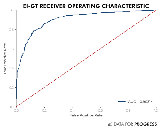
This series of graphs compare the performance of the EI model and the VR model on two datasets. The first graph on the left compares the EI model’s individual predictions to the synthetic vote choice on the Florida dataset. Here the EI model is basically perfect, as is clear from the AUC (AUC is a measure of how good a binary classifier is, the closer to one the closest to a perfect classifier). That’s really good; it means the EI model is essentially learning all of the complexities embedded in the VR model. Maybe even more impressive though, the next two graphs compare the performance of the EI model and the VR model on our linked survey data; the data we used to train the VR model in the first place. In the center is the ROC curve for the VR model on the polling data, where it achieves 82% accuracy and an AUC of 0.90245; the VR model should be doing pretty well on this data, it was trained on this data. On the right, we have the ROC curve for the EI model on the survey data, and that’s where it gets very interesting. The EI model does better than the original VR model (achieving an accuracy of 83% and an AUC of 0.90314) even though the VR model was trained on this survey dataset while the EI model was only trained on the synthetic Florida data!
This result confirms that the EI method is very likely applicable to real-world voting problems. It is not without limitations though, several major questions remain open. First is a simple question of whether it is the sheer scale of the Florida data that allows the EI model to be so effective here. It may be that for smaller geographies the model works less well. Second is a question of local effects; precinct-level interactions may be significant in predicting votes. Normally precinct-level variables can be added to the model to account for these impacts, but in the EI framework, this will likely prevent the model from learning the underlying relationships. It is unclear how large an issue this will be, and the precinct level calibration technique discussed in the previous post may resolve this issue.
We will explore these two questions in the next couple of blog posts in this series.
Colin McAuliffe (@ColinJMcAuliffe) is a co-founder of Data for Progress.
Nic Fishman (@njwfish) is a senior advisor to Data for Progress.