Inferring Vote Choice Without a Survey

By Colin McAuliffe (@ColinJMcAuliffe) and Ryan O’Donnell (@RyanODonnellPA)

Interpreting election results is tricky because there is no way to know for sure exactly which voters voted for which candidates. Exit polls and other types of surveys are useful, but come with disadvantages and often are only available for a few high profile races. Another option is to analyze aggregate data such a precinct level results, where precinct characteristics are used in regressions on the aggregate vote share of a candidate. This also has problems, primarily from the fact that it is often misleading to attempt to draw conclusions about individual behavior from aggregated information.

This post outlines another option, where an individual-level model for candidate choice is fit to precinct level voting data. This is made possible by a voter file, which contains records of who voted in each election along with various characteristics about them -- including which precinct they live in. The nice thing about this method is that a survey isn’t needed (although a survey could be incorporated if one is available), and the model is constructed at the individual-level as opposed to the aggregate-level. This partially alleviates some of the problems that arise from working with aggregated data, although we are still stuck with aggregated vote choice data. Ideally, we would like to use survey data in conjunction with election returns to understand the electorate, as other organizations have done. However, we contend that our method is substantially better than analyzing aggregated data for instances where surveys are not available.

First, we have a set of individual level covariates that are available in the voter which we want to include in our model, so that $X$_$ji$ is a covariate $j$ for person $i$, who lives in precinct $a(i)$. A linear model for the probability that person i voted for the primary challenger is:

Where $\alpha$ is a common interecept and $\beta_j$ is a paramter associated with the effect of covariate $j$. The sigmoid function transforms the model output so that it is constrained between 0 and 1.

In an ideal world we would have observations on the individual level to fit the model parameters, but this time, we only have results at the precinct level, so we need a way to link our model to those observations. The way we do this is to compute the average probability of voting for the challenger in each precinct. From a computational standpoint, it’s convenient and efficient to apply the average with a sparse indicator matrix as follows:

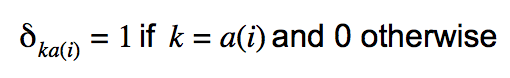
For person $i$ in precinct $a(i)$, and precinct $k$ containing $n_k$ voters, let

Where

Then, the precinct average of the individual probabilities $\pi_k$ can be computed with a sparse matrix-vector multiplication

With the average probabilities, we can specify a binomial distribution for the number of votes won by the challenger $v_k$ given the total number of votes in the precint $n_k$ $$v_k\sim Binomial(\pi_k,n_k)$$ Comparing this model to a model that uses aggregate data makes the differences clear. For an aggregate model, instead of covariates associated with individuals, we have precinct level covariates $D$_$kq$. This directly gives us an average precinct level probability of voting for the challenger.

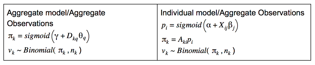
While the individual model requires a fairly large amount of additional computation relative to the aggregate model, we also gain substantial amounts of information which simply can not be obtained using the aggregate model. With the aggregate model, the best we can do is assign a uniform probability of voting for the challenger $\pi_k$ to everyone in a precinct, but the individual model allows us to leverage trends in demographic sorting and vote share by precinct to capture within-precinct heterogeneity in the support probabilities.

Additionally, since the vote tallies represent a population instead of a sample, we can use them to calibrate the model’s predictions. We observe $v_k$ votes for the challenger in precinct $k$, but the model will typically not predict exactly that many votes. Therefore, we take the $v_k$ voters with the highest support probabilities and assign their vote to the challenger. We repeat this process for each draw from the posterior predictive distribution of $p_i$ to get a sense of uncertainty in our estimated vote choice estimates.

We’ll use Ayanna Pressley’s MA-7 primary in 2018 as an example. Our model uses covariates such as age, general and primary turnout history, gender, education, and registration date. Below, we show how the uncalibrated model predictions with the actual results. The uncalibrated individual support probabilities do a reasonable job of matching with the observed results. After we calibrate the model by adjusting the raw support probabilities, all the points on the plot below fall on a straight line (more details on this type of calibration can be found here and here). To be clear, while the calibrated support probabilities match observations exactly in aggregate, this does not guarantee that our individual vote choice estimates are correct and uncertainty about those estimates still remains. Uncertainty is an inherent characteristic of inverse problems in general, which require the analyst to make many assumptions which are not subject to direct empirical verification.

Individual level estimates of vote choice are hugely valuable since now we can create crosstabs and other summaries of candidate support – which allows us to better estimate how candidates won their race. For example, we can compare how Ayanna Pressley performed compared to Mike Capuano by race.

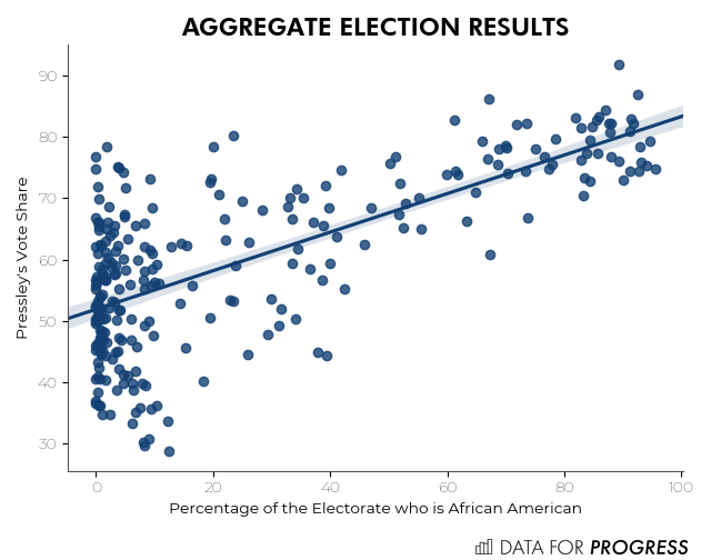
In this case, the aggregate results tell a similar story to the individual results. A simple plot of Pressley’s vote share against the percentage of a precinct’s electorate that is African American suggests that Pressley had strong support from African American voters.

It’s much harder to extract information about age through aggregate measures however, comparing Pressley’s vote share to the proportion of the electorate that’s over 50 doesn’t reveal much of a trend.

Accounting for more variables in an aggregate regression model could help us dig deeper, but generally it’s not easy to come up with an aggregate metric for age that will be informative of how age is related to voting patterns. Since the individual-level model uses age at the individual level, this isn’t a problem and we uncover a pretty striking trend showing strong support for Pressley among younger voters.

We’ll be using this method to explore patterns in a number of recent primaries and general elections, so stay tuned for more to come.

Colin McAuliffe (@ColinJMcAuliffe) is a cofounder of Data for Progress.

Ryan O’Donnell (@RyanODonnellPA) is a senior advisor for Data for Progress.